Simulation of a mixture model

Simulation of the mixture model, with estimation of the integration error.

Michel Bierlaire, EPFL Fri Jun 20 2025, 10:29:35

import sys

import numpy as np
from biogeme.biogeme import BIOGEME
from biogeme.expressions import Beta, Draws, MonteCarlo
from biogeme.models import logit
from biogeme.results_processing import EstimationResults

See the data processing script: Data preparation for Swissmetro.

from swissmetro_data import (
    CAR_AV_SP,
    CAR_CO_SCALED,
    CAR_TT_SCALED,
    CHOICE,
    SM_AV,
    SM_COST_SCALED,
    SM_TT_SCALED,
    TRAIN_AV_SP,
    TRAIN_COST_SCALED,
    TRAIN_TT_SCALED,
    database,
)

try:
    import matplotlib.pyplot as plt

    PLOT = True
except ModuleNotFoundError:
    print('Install matplotlib to see the distribution of integration errors.')
    print('pip install matplotlib')
    PLOT = False

Parameters to be estimated.

asc_car = Beta('asc_car', 0, None, None, 0)
asc_train = Beta('asc_train', 0, None, None, 0)
asc_sm = Beta('asc_sm', 0, None, None, 1)
b_cost = Beta('b_cost', 0, None, None, 0)

Define a random parameter, normally distributed, designed to be used for Monte-Carlo simulation.

b_time = Beta('b_time', 0, None, None, 0)

It is advised not to use 0 as starting value for the following parameter.

b_time_s = Beta('b_time_s', 1, None, None, 0)
b_time_rnd = b_time + b_time_s * Draws('b_time_rnd', 'NORMAL')

Definition of the utility functions.

v_train = asc_train + b_time_rnd * TRAIN_TT_SCALED + b_cost * TRAIN_COST_SCALED
v_swissmetro = asc_sm + b_time_rnd * SM_TT_SCALED + b_cost * SM_COST_SCALED
v_car = asc_car + b_time_rnd * CAR_TT_SCALED + b_cost * CAR_CO_SCALED

Associate utility functions with the numbering of alternatives.

v = {1: v_train, 2: v_swissmetro, 3: v_car}

Associate the availability conditions with the alternatives.

av = {1: TRAIN_AV_SP, 2: SM_AV, 3: CAR_AV_SP}

The estimation results are read from the pickle file.

try:
    results = EstimationResults.from_yaml_file(
        filename='saved_results/b05normal_mixture.yaml'
    )
except FileNotFoundError:
    print(
        'Run first the script plot_b05normal_mixture.py in order to generate the '
        'file b05normal_mixture.yaml.'
    )
    sys.exit()

Conditional to b_time_rnd, we have a logit model (called the kernel)

conditional_probability = logit(v, av, CHOICE)

We calculate the integration error. Note that this formula assumes independent draws, and is not valid for Halton or antithetic draws.

integral = MonteCarlo(conditional_probability)
integral_square = MonteCarlo(conditional_probability * conditional_probability)
variance = integral_square - integral * integral
error = (variance / 2.0) ** 0.5

And the value of the individual parameters.

numerator = MonteCarlo(b_time_rnd * conditional_probability)
denominator = integral

simulate = {
    'Numerator': numerator,
    'Denominator': denominator,
    'Integral': integral,
    'Integration error': error,
}

Create the Biogeme object.

biosim = BIOGEME(database, simulate, number_of_draws=10000)
biosim.model_name = 'b05normal_mixture_simul'

NUmber of draws

print(f'Number of draws: {biosim.number_of_draws}')

Number of draws: 10000

Simulate the requested quantities. The output is a Pandas data frame.

simulation_results = biosim.simulate(results.get_beta_values())

95% confidence interval on the log likelihood.

simulation_results['left'] = np.log(
    simulation_results['Integral'] - 1.96 * simulation_results['Integration error']
)
simulation_results['right'] = np.log(
    simulation_results['Integral'] + 1.96 * simulation_results['Integration error']
)

/Users/bierlair/python_envs/venv313/lib/python3.13/site-packages/pandas/core/arraylike.py:399: RuntimeWarning: invalid value encountered in log
  result = getattr(ufunc, method)(*inputs, **kwargs)

print(f'Log likelihood: {np.log(simulation_results["Integral"]).sum()}')

Log likelihood: -5214.689681629532

print(
    f'Integration error for {biosim.number_of_draws} draws: '
    f'{simulation_results["Integration error"].sum()}'
)

Integration error for 10000 draws: 716.8094872624056

print(f'In average {simulation_results["Integration error"].mean()} per observation.')

In average 0.1059115672669039 per observation.

95% confidence interval

print(
    f'95% confidence interval: [{simulation_results["left"].sum()} - '
    f'{simulation_results["right"].sum()}]'
)

95% confidence interval: [-7583.2407468481015 - -2719.046943930449]

Post processing to obtain the individual parameters.

simulation_results['Beta'] = (
    simulation_results['Numerator'] / simulation_results['Denominator']
)

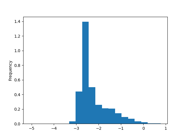
Plot the histogram of individual parameters

if PLOT:
    simulation_results['Beta'].plot(kind='hist', density=True, bins=20)

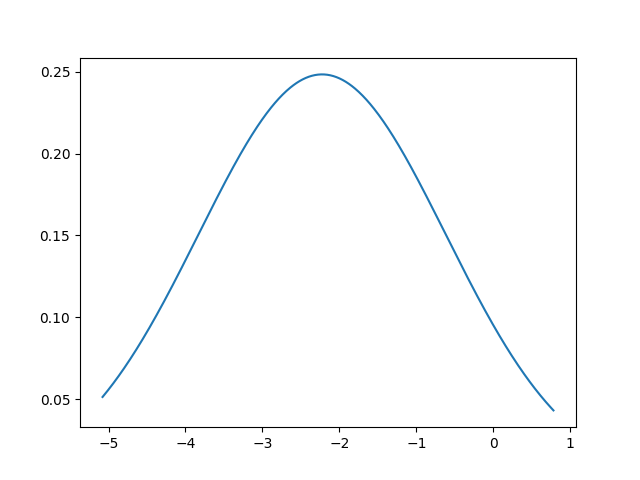
Plot the general distribution of Beta

def normalpdf(val: float, mu: float = 0.0, std: float = 1.0) -> float:
    """
    Calculate the pdf of the normal distribution, for plotting purposes.

    """
    d = -(val - mu) * (val - mu)
    n = 2.0 * std * std
    a = d / n
    num = np.exp(a)
    den = std * 2.506628275
    p = num / den
    return p

betas = results.get_beta_values(['b_time', 'b_time_s'])
x = np.arange(simulation_results['Beta'].min(), simulation_results['Beta'].max(), 0.01)

if PLOT:
    plt.plot(x, normalpdf(x, betas['b_time'], betas['b_time_s']), '-')
    plt.show()