Examples of mathematical expressions

Example of manipulating mathematical expressions and calculation of derivatives.

Michel Bierlaire, EPFL Sat Jun 28 2025, 15:54:00

import numpy as np

from biogeme.calculator import (
    CallableExpression,
    create_function_simple_expression,
    get_value_and_derivatives,
)
from biogeme.function_output import FunctionOutput, NamedFunctionOutput

try:
    import matplotlib.pyplot as plt

    can_plot = True
except ModuleNotFoundError:
    can_plot = False


from biogeme.expressions import Beta, exp

# ##
# We create a simple expression:
b = Beta('b', 1, None, None, 0)
expression = exp(-b * b + 1)

We can calculate its value. Note that, as the expression is calculated out of Biogeme, the IDs must be prepared. So the parameter ‘prepare_ids’ is set to True

z = expression.get_value()
print(f'exp(-b * b + 1) = {z}')

exp(-b * b + 1) = 1.0

We can also calculate the value, the first derivative, the second derivative, and the BHHH, which in this case is the square of the first derivatives

the_function_output: FunctionOutput = get_value_and_derivatives(
    expression, numerically_safe=False, use_jit=True
)

print(f'f = {the_function_output.function}')

f = 1.0

print(f'g = {the_function_output.gradient}')

g = [-2.]

print(f'h = {the_function_output.hessian}')

h = [[2.]]

print(f'BHHH = {the_function_output.bhhh}')

BHHH = [[4.]]

From the expression, we can create a Python function that takes as argument the value of the free parameters, and returns the function, the first, the second derivatives, and the BHHH.

fct: CallableExpression = create_function_simple_expression(
    expression, numerically_safe=False, named_output=True, use_jit=True
)

By default, we want to calculate the gradient and the hessian

def the_function(x: float) -> NamedFunctionOutput:
    # The generated function takes an array of betas as argument. In this example, there is only one.
    beta = [x]
    return fct(beta, gradient=True, hessian=True, bhhh=False)

We can use the function for different values of the parameter. Note that it takes as argument a vector of betas.

beta = 2.0
the_named_function_output: NamedFunctionOutput = the_function(beta)
print(f'f({beta}) = {the_named_function_output.function}')
print(f'g({beta}) = {the_named_function_output.gradient}')
print(f'h({beta}) = {the_named_function_output.hessian}')

f(2.0) = 0.049787068367863944
g(2.0) = {'b': np.float64(-0.19914827347145578)}
h(2.0) = {'b': {'b': np.float64(0.6970189571500952)}}

beta = 3.0
the_named_function_output = the_function(beta)
print(f'f({beta}) = {the_named_function_output.function}')
print(f'g({beta}) = {the_named_function_output.gradient}')
print(f'h({beta}) = {the_named_function_output.hessian}')

f(3.0) = 0.00033546262790251185
g(3.0) = {'b': np.float64(-0.0020127757674150712)}
h(3.0) = {'b': {'b': np.float64(0.011405729348685403)}}

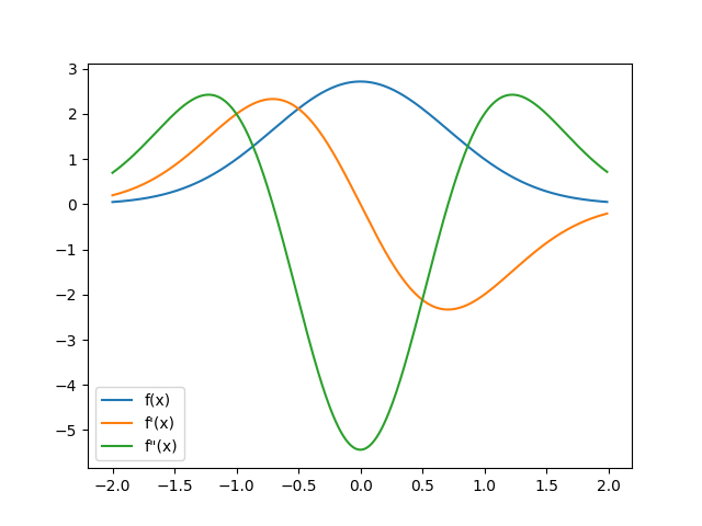
if can_plot:
    # We can also use it to plot the function and its derivatives
    x = np.arange(-2, 2, 0.1)

    # The value of the function.
    f = [the_function(xx).function for xx in x]

    # The gradient is element [1]. As it contains only one entry [0],
    # we convert it into float.

    g = [float(the_function(xx).gradient['b']) for xx in x]

    # The hessian is element [2]. As it contains only one entry
    # [0][0], we convert it into float.
    h = [float(the_function(xx).hessian['b']['b']) for xx in x]

    ax = plt.gca()
    ax.plot(x, f, label="f(x)")
    ax.plot(x, g, label="f'(x)")
    ax.plot(x, h, label='f"(x)')
    ax.legend()

    plt.show()