Calculation of revenues

We use an estimated model to calculate revenues.

author:

Michel Bierlaire, EPFL

date:

Wed Apr 12 21:02:19 2023

import sys
import numpy as np

try:
    import matplotlib.pyplot as plt

    can_plot = True
except ModuleNotFoundError:
    can_plot = False
from tqdm import tqdm
from biogeme import models
import biogeme.exceptions as excep
import biogeme.biogeme as bio
import biogeme.results as res
from optima_data import database, normalized_weight
from scenarios import scenario

Read the estimation results from the file.

try:
    results = res.bioResults(pickleFile='saved_results/b02estimation.pickle')
except excep.BiogemeError:
    sys.exit(
        'Run first the script b02simulation.py '
        'in order to generate the '
        'file b02estimation.pickle.'
    )

Function calculating the revenues

def revenues(factor: float) -> tuple[float, float, float]:
    """Calculate the total revenues generated by public transportation,
        when the price is multiplied by a factor.

    :param factor: factor that multiplies the current cost of public
        transportation

    :return: total revenues, followed by the lower and upper bound of
        the confidence interval.

    """
    # Obtain the specification for the default scenario
    V, nests, _, marginal_cost_scenario = scenario(factor=factor)

    # Obtain the expression for the choice probability of each alternative
    prob_pt = models.nested(V, None, nests, 0)

    # We now simulate the choice probabilities,the weight and the
    # price variable

    simulate = {
        'weight': normalized_weight,
        'Revenue public transportation': prob_pt * marginal_cost_scenario,
    }

    the_biogeme = bio.BIOGEME(database, simulate)
    simulated_values = the_biogeme.simulate(results.getBetaValues())

    # We also calculate confidence intervals for the calculated quantities

    betas = the_biogeme.free_beta_names()
    beta_bootstrap = results.getBetasForSensitivityAnalysis(betas)
    left, right = the_biogeme.confidenceIntervals(beta_bootstrap, 0.9)

    revenues_pt = (
        simulated_values['Revenue public transportation'] * simulated_values['weight']
    ).sum()
    revenues_pt_left = (left['Revenue public transportation'] * left['weight']).sum()
    revenues_pt_right = (right['Revenue public transportation'] * right['weight']).sum()
    return revenues_pt, revenues_pt_left, revenues_pt_right

Current revenues for public transportation

r, r_left, r_right = revenues(factor=1.0)
print(
    f'Total revenues for public transportation (for the sample): {r:.1f} CHF '
    f'[{r_left:.1f} CHF, '
    f'{r_right:.1f} CHF]'
)

Total revenues for public transportation (for the sample): 3018.3 CHF [2418.8 CHF, 3683.3 CHF]

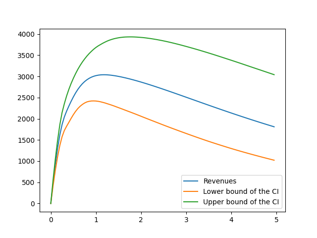
We now investigate how the revenues vary with the multiplicative factor

factors = np.arange(0.0, 5.0, 0.05)
plot_revenues = [revenues(s) for s in tqdm(factors)]
zipped = zip(*plot_revenues)
rev = next(zipped)
lower = next(zipped)
upper = next(zipped)

largest_revenue = max(rev)
max_index = rev.index(largest_revenue)

  0%|          | 0/100 [00:00<?, ?it/s]
  1%|          | 1/100 [00:06<09:59,  6.06s/it]
  2%|▏         | 2/100 [00:12<09:54,  6.06s/it]
  3%|▎         | 3/100 [00:18<09:47,  6.06s/it]
  4%|▍         | 4/100 [00:24<09:42,  6.07s/it]
  5%|▌         | 5/100 [00:30<09:36,  6.07s/it]
  6%|▌         | 6/100 [00:36<09:30,  6.07s/it]
  7%|▋         | 7/100 [00:42<09:23,  6.06s/it]
  8%|▊         | 8/100 [00:48<09:17,  6.06s/it]
  9%|▉         | 9/100 [00:54<09:12,  6.07s/it]
 10%|█         | 10/100 [01:00<09:06,  6.08s/it]
 11%|█         | 11/100 [01:06<09:01,  6.08s/it]
 12%|█▏        | 12/100 [01:12<08:55,  6.08s/it]
 13%|█▎        | 13/100 [01:18<08:48,  6.08s/it]
 14%|█▍        | 14/100 [01:25<08:43,  6.08s/it]
 15%|█▌        | 15/100 [01:31<08:37,  6.09s/it]
 16%|█▌        | 16/100 [01:37<08:31,  6.09s/it]
 17%|█▋        | 17/100 [01:43<08:26,  6.10s/it]
 18%|█▊        | 18/100 [01:49<08:20,  6.10s/it]
 19%|█▉        | 19/100 [01:55<08:17,  6.15s/it]
 20%|██        | 20/100 [02:01<08:11,  6.14s/it]
 21%|██        | 21/100 [02:07<08:00,  6.09s/it]
 22%|██▏       | 22/100 [02:13<07:52,  6.06s/it]
 23%|██▎       | 23/100 [02:19<07:47,  6.07s/it]
 24%|██▍       | 24/100 [02:26<07:44,  6.11s/it]
 25%|██▌       | 25/100 [02:32<07:37,  6.10s/it]
 26%|██▌       | 26/100 [02:38<07:33,  6.13s/it]
 27%|██▋       | 27/100 [02:44<07:26,  6.12s/it]
 28%|██▊       | 28/100 [02:50<07:20,  6.12s/it]
 29%|██▉       | 29/100 [02:56<07:16,  6.15s/it]
 30%|███       | 30/100 [03:03<07:13,  6.19s/it]
 31%|███       | 31/100 [03:09<07:09,  6.22s/it]
 32%|███▏      | 32/100 [03:15<07:03,  6.23s/it]
 33%|███▎      | 33/100 [03:21<06:54,  6.18s/it]
 34%|███▍      | 34/100 [03:27<06:44,  6.13s/it]
 35%|███▌      | 35/100 [03:33<06:38,  6.13s/it]
 36%|███▌      | 36/100 [03:39<06:30,  6.11s/it]
 37%|███▋      | 37/100 [03:45<06:24,  6.11s/it]
 38%|███▊      | 38/100 [03:52<06:21,  6.16s/it]
 39%|███▉      | 39/100 [03:58<06:15,  6.15s/it]
 40%|████      | 40/100 [04:04<06:09,  6.16s/it]
 41%|████      | 41/100 [04:10<06:02,  6.14s/it]
 42%|████▏     | 42/100 [04:16<05:55,  6.13s/it]
 43%|████▎     | 43/100 [04:22<05:49,  6.13s/it]
 44%|████▍     | 44/100 [04:29<05:43,  6.13s/it]
 45%|████▌     | 45/100 [04:35<05:35,  6.10s/it]
 46%|████▌     | 46/100 [04:41<05:30,  6.12s/it]
 47%|████▋     | 47/100 [04:47<05:23,  6.11s/it]
 48%|████▊     | 48/100 [04:53<05:17,  6.11s/it]
 49%|████▉     | 49/100 [04:59<05:11,  6.10s/it]
 50%|█████     | 50/100 [05:05<05:05,  6.10s/it]
 51%|█████     | 51/100 [05:11<04:58,  6.10s/it]
 52%|█████▏    | 52/100 [05:17<04:52,  6.09s/it]
 53%|█████▎    | 53/100 [05:23<04:46,  6.09s/it]
 54%|█████▍    | 54/100 [05:29<04:40,  6.09s/it]
 55%|█████▌    | 55/100 [05:36<04:34,  6.11s/it]
 56%|█████▌    | 56/100 [05:42<04:28,  6.10s/it]
 57%|█████▋    | 57/100 [05:48<04:22,  6.10s/it]
 58%|█████▊    | 58/100 [05:54<04:16,  6.11s/it]
 59%|█████▉    | 59/100 [06:00<04:10,  6.10s/it]
 60%|██████    | 60/100 [06:06<04:04,  6.12s/it]
 61%|██████    | 61/100 [06:12<03:58,  6.11s/it]
 62%|██████▏   | 62/100 [06:18<03:51,  6.10s/it]
 63%|██████▎   | 63/100 [06:24<03:45,  6.10s/it]
 64%|██████▍   | 64/100 [06:31<03:40,  6.12s/it]
 65%|██████▌   | 65/100 [06:37<03:34,  6.11s/it]
 66%|██████▌   | 66/100 [06:43<03:27,  6.11s/it]
 67%|██████▋   | 67/100 [06:49<03:20,  6.09s/it]
 68%|██████▊   | 68/100 [06:55<03:14,  6.09s/it]
 69%|██████▉   | 69/100 [07:01<03:10,  6.15s/it]
 70%|███████   | 70/100 [07:07<03:04,  6.14s/it]
 71%|███████   | 71/100 [07:13<02:57,  6.12s/it]
 72%|███████▏  | 72/100 [07:19<02:51,  6.11s/it]
 73%|███████▎  | 73/100 [07:26<02:44,  6.11s/it]
 74%|███████▍  | 74/100 [07:32<02:38,  6.11s/it]
 75%|███████▌  | 75/100 [07:38<02:32,  6.11s/it]
 76%|███████▌  | 76/100 [07:44<02:26,  6.11s/it]
 77%|███████▋  | 77/100 [07:50<02:20,  6.10s/it]
 78%|███████▊  | 78/100 [07:56<02:14,  6.11s/it]
 79%|███████▉  | 79/100 [08:02<02:08,  6.12s/it]
 80%|████████  | 80/100 [08:09<02:03,  6.16s/it]
 81%|████████  | 81/100 [08:15<01:57,  6.19s/it]
 82%|████████▏ | 82/100 [08:21<01:51,  6.21s/it]
 83%|████████▎ | 83/100 [08:27<01:45,  6.23s/it]
 84%|████████▍ | 84/100 [08:34<01:39,  6.25s/it]
 85%|████████▌ | 85/100 [08:40<01:33,  6.26s/it]
 86%|████████▌ | 86/100 [08:46<01:27,  6.26s/it]
 87%|████████▋ | 87/100 [08:52<01:21,  6.26s/it]
 88%|████████▊ | 88/100 [08:59<01:15,  6.27s/it]
 89%|████████▉ | 89/100 [09:05<01:09,  6.32s/it]
 90%|█████████ | 90/100 [09:11<01:03,  6.30s/it]
 91%|█████████ | 91/100 [09:18<00:56,  6.29s/it]
 92%|█████████▏| 92/100 [09:24<00:50,  6.29s/it]
 93%|█████████▎| 93/100 [09:30<00:44,  6.30s/it]
 94%|█████████▍| 94/100 [09:37<00:38,  6.47s/it]
 95%|█████████▌| 95/100 [09:45<00:34,  6.94s/it]
 96%|█████████▌| 96/100 [09:52<00:27,  6.96s/it]
 97%|█████████▋| 97/100 [09:58<00:20,  6.74s/it]
 98%|█████████▊| 98/100 [10:05<00:13,  6.59s/it]
 99%|█████████▉| 99/100 [10:11<00:06,  6.50s/it]
100%|██████████| 100/100 [10:17<00:00,  6.43s/it]
100%|██████████| 100/100 [10:17<00:00,  6.18s/it]

print(
    f'Largest revenue: {largest_revenue:.1f} obtained with '
    f'factor {factors[max_index]:.1f}'
)

Largest revenue: 3039.0 obtained with factor 1.2

if can_plot:
    # We plot the results
    ax = plt.gca()
    ax.plot(factors, rev, label="Revenues")
    ax.plot(factors, lower, label="Lower bound of the CI")
    ax.plot(factors, upper, label="Upper bound of the CI")
    ax.legend()

    plt.show()