Re-estimate the Pareto optimal models

The assisted specification algorithm generates a file containg the pareto optimal specification. This script is designed to re-estimate the Pareto optimal models. The catalog of specifications is defined in Specification of a catalog of models .

author:

Michel Bierlaire, EPFL

date:

Wed Apr 12 17:25:41 2023

try:
    import matplotlib.pyplot as plt

    can_plot = True
except ModuleNotFoundError:
    can_plot = False
from biogeme.assisted import ParetoPostProcessing
from biogeme.results import compileEstimationResults
from plot_b22multiple_models_spec import the_biogeme

PARETO_FILE_NAME = 'saved_results/b22multiple_models.pareto'

CSV_FILE = 'b22process_pareto.csv'
SEP_CSV = ','

The constructor of the Pareto post processing object takes two arguments:

• the biogeme object,

• the name of the file where the algorithm has stored the estimated models.

the_pareto_post = ParetoPostProcessing(
    biogeme_object=the_biogeme,
    pareto_file_name=PARETO_FILE_NAME,
)

the_pareto_post.log_statistics()

all_results = the_pareto_post.reestimate(recycle=True)

summary, description = compileEstimationResults(all_results, use_short_names=True)
print(summary)

                                   Model_000000     Model_000001     Model_000002     Model_000003       Model_000004       Model_000005
Number of estimated parameters                6                8                4                9                  7                 10
Sample size                                6768             6768             6768             6768               6768               6768
Final log likelihood               -5003.527151     -4830.277686     -5245.757762     -4823.005819       -4932.510059       -4802.769989
Akaike Information Criterion       10019.054301      9676.555372     10499.515524      9664.011638        9879.020118        9625.539979
Bayesian Information Criterion     10059.974067       9731.11506     10526.795368      9725.391287        9926.759844        9693.739588
ASC_CAR (t-test)                -0.359  (-5.21)  -0.553  (-5.26)  0.0519  (0.954)  -0.564  (-5.39)    -0.282  (-4.81)    -0.696  (-6.55)
ASC_CAR_with_ga (t-test)         -1.86  (-9.51)      -2  (-9.34)                    -2.02  (-9.53)     -1.83  (-8.98)        -2  (-9.46)
ASC_TRAIN (t-test)               -1.48  (-15.6)  -0.375  (-4.12)  -0.505  (-6.92)  -0.386  (-4.24)    -0.918  (-10.6)  -0.0737  (-0.703)
ASC_TRAIN_with_ga (t-test)         2.08  (23.4)     2.13  (23.5)                      2.08  (22.4)       2.24  (25.3)       2.11  (22.5)
B_COST (t-test)                  -1.45  (-17.9)    -1.5  (-18.4)   -2.35  (-18.3)   -1.49  (-18.1)      -1.5  (-18.2)     -1.49  (-18.1)
B_TIME (t-test)                  -1.03  (-10.1)   -1.63  (-20.4)   -3.32  (-18.3)   -1.62  (-20.1)     -1.59  (-20.3)       -1.61  (-20)
ASC_CAR_male (t-test)                               0.46  (4.26)                      0.48  (4.41)                         0.474  (4.36)
ASC_TRAIN_male (t-test)                           -1.17  (-13.9)                    -1.14  (-13.4)                        -1.16  (-13.5)
lambda_TT (t-test)                                                                   0.219  (3.06)                         0.223  (3.12)
B_HEADWAY (t-test)                                                                                  -0.00612  (-5.82)  -0.00664  (-6.12)

print(f'Summary table available in {CSV_FILE}')
summary.to_csv(CSV_FILE, sep=SEP_CSV)

Summary table available in b22process_pareto.csv

Explanation of the short names of the models.

with open(CSV_FILE, 'a', encoding='utf-8') as f:
    print('\n\n', file=f)
    for k, v in description.items():
        if k != v:
            print(f'{k}: {v}')
            print(f'{k}{SEP_CSV}{v}', file=f)

Model_000000: ASC:MALE-GA;TRAIN_COST_catalog:log;TRAIN_HEADWAY_catalog:with_headway;TRAIN_TT_catalog:log
Model_000001: ASC:no_seg;TRAIN_COST_catalog:sqrt;TRAIN_HEADWAY_catalog:without_headway;TRAIN_TT_catalog:sqrt
Model_000002: ASC:GA;TRAIN_COST_catalog:sqrt;TRAIN_HEADWAY_catalog:without_headway;TRAIN_TT_catalog:sqrt
Model_000003: ASC:MALE-GA;TRAIN_COST_catalog:sqrt;TRAIN_HEADWAY_catalog:without_headway;TRAIN_TT_catalog:sqrt
Model_000004: ASC:GA;TRAIN_COST_catalog:log;TRAIN_HEADWAY_catalog:with_headway;TRAIN_TT_catalog:log
Model_000005: ASC:MALE-GA;TRAIN_COST_catalog:log;TRAIN_HEADWAY_catalog:with_headway;TRAIN_TT_catalog:boxcox

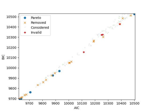
The following plot illustrates all models that have been estimated. Each dot corresponds to a model. The x-coordinate corresponds to the Akaike Information Criterion (AIC). The y-coordinate corresponds to the Bayesian Information Criterion (BIC). Note that there is a third objective that does not appear on this picture: the number of parameters. If the shape of the dot is a circle, it means that it corresponds to a Pareto optimal model. If the shape is a cross, it means that the model has been Pareto optimal at some point during the algorithm and later removed as a new model dominating it has been found. If the shape is a start, it means that the model has been deemed invalid.

if can_plot:
    _ = the_pareto_post.plot(label_x='AIC', label_y='BIC')
    plt.show()

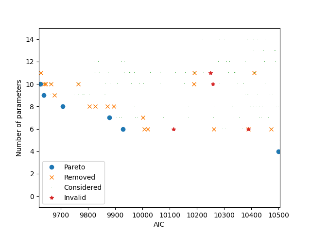
It is possible to plot two different objectives: AIC and number of parameters.

if can_plot:
    _ = the_pareto_post.plot(
        objective_x=0, objective_y=2, label_x='AIC', label_y='Number of parameters'
    )
    plt.show()

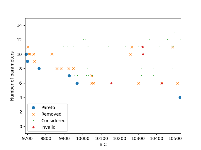
It is possible to plot two different objectives: BIC and number of parameters.

if can_plot:
    _ = the_pareto_post.plot(
        objective_x=1, objective_y=2, label_x='BIC', label_y='Number of parameters'
    )
    plt.show()