Re-estimate the Pareto optimal models

The assisted specification algorithm generates a file containg the pareto optimal specification. This script is designed to re-estimate the Pareto optimal models. The catalog of specifications is defined in Specification of a catalog of models .

author:

Michel Bierlaire, EPFL

date:

Wed Apr 12 17:46:14 2023

import biogeme.biogeme_logging as blog

try:
    import matplotlib.pyplot as plt

    can_plot = True
except ModuleNotFoundError:
    can_plot = False
from biogeme_optimization.exceptions import OptimizationError
from biogeme.assisted import ParetoPostProcessing
from biogeme.results import compileEstimationResults
from plot_b21multiple_models_spec import the_biogeme

PARETO_FILE_NAME = 'saved_results/b21multiple_models.pareto'

logger = blog.get_screen_logger(blog.INFO)
logger.info('Example b21process_pareto.py')

CSV_FILE = 'b21process_pareto.csv'
SEP_CSV = ','

Example b21process_pareto.py

The constructor of the Pareto post processing object takes two arguments:

• the biogeme object,

• the name of the file where the algorithm has stored the estimated models.

the_pareto_post = ParetoPostProcessing(
    biogeme_object=the_biogeme,
    pareto_file_name=PARETO_FILE_NAME,
)

Pareto set initialized from file with 36 elements [8 Pareto] and 0 invalid elements.

the_pareto_post.log_statistics()

Pareto: 8
Condidered: 36
Removed: 4

Complete re-estimation of the best models, including the calculation of the statistics.

all_results = the_pareto_post.reestimate(recycle=False)

File biogeme.toml has been parsed.
*** Initial values of the parameters are obtained from the file __b21multiple_models_000000.iter
Parameter values restored from __b21multiple_models_000000.iter
Optimization algorithm: hybrid Newton/BFGS with simple bounds [simple_bounds]
** Optimization: Newton with trust region for simple bounds
Results saved in file b21multiple_models_000000~00.html
Results saved in file b21multiple_models_000000~00.pickle
File biogeme.toml has been parsed.
*** Initial values of the parameters are obtained from the file __b21multiple_models_000001.iter
Parameter values restored from __b21multiple_models_000001.iter
Optimization algorithm: hybrid Newton/BFGS with simple bounds [simple_bounds]
** Optimization: Newton with trust region for simple bounds
Results saved in file b21multiple_models_000001~00.html
Results saved in file b21multiple_models_000001~00.pickle
File biogeme.toml has been parsed.
*** Initial values of the parameters are obtained from the file __b21multiple_models_000002.iter
Parameter values restored from __b21multiple_models_000002.iter
Optimization algorithm: hybrid Newton/BFGS with simple bounds [simple_bounds]
** Optimization: Newton with trust region for simple bounds
Results saved in file b21multiple_models_000002~00.html
Results saved in file b21multiple_models_000002~00.pickle
File biogeme.toml has been parsed.
*** Initial values of the parameters are obtained from the file __b21multiple_models_000003.iter
Parameter values restored from __b21multiple_models_000003.iter
Optimization algorithm: hybrid Newton/BFGS with simple bounds [simple_bounds]
** Optimization: Newton with trust region for simple bounds
Results saved in file b21multiple_models_000003~00.html
Results saved in file b21multiple_models_000003~00.pickle
File biogeme.toml has been parsed.
*** Initial values of the parameters are obtained from the file __b21multiple_models_000004.iter
Parameter values restored from __b21multiple_models_000004.iter
Optimization algorithm: hybrid Newton/BFGS with simple bounds [simple_bounds]
** Optimization: Newton with trust region for simple bounds
Results saved in file b21multiple_models_000004~00.html
Results saved in file b21multiple_models_000004~00.pickle
File biogeme.toml has been parsed.
*** Initial values of the parameters are obtained from the file __b21multiple_models_000005.iter
Parameter values restored from __b21multiple_models_000005.iter
Optimization algorithm: hybrid Newton/BFGS with simple bounds [simple_bounds]
** Optimization: Newton with trust region for simple bounds
Results saved in file b21multiple_models_000005~00.html
Results saved in file b21multiple_models_000005~00.pickle
File biogeme.toml has been parsed.
*** Initial values of the parameters are obtained from the file __b21multiple_models_000006.iter
Parameter values restored from __b21multiple_models_000006.iter
Optimization algorithm: hybrid Newton/BFGS with simple bounds [simple_bounds]
** Optimization: Newton with trust region for simple bounds
Results saved in file b21multiple_models_000006~00.html
Results saved in file b21multiple_models_000006~00.pickle
File biogeme.toml has been parsed.
*** Initial values of the parameters are obtained from the file __b21multiple_models_000007.iter
Parameter values restored from __b21multiple_models_000007.iter
Optimization algorithm: hybrid Newton/BFGS with simple bounds [simple_bounds]
** Optimization: Newton with trust region for simple bounds
Results saved in file b21multiple_models_000007~00.html
Results saved in file b21multiple_models_000007~00.pickle

summary, description = compileEstimationResults(all_results, use_short_names=True)
print(summary)

The syntax "compileEstimationResults" is deprecated and is replaced by the syntax "compile_estimation_results".
                                   Model_000000     Model_000001     Model_000002      Model_000003     Model_000004         Model_000005     Model_000006     Model_000007
Number of estimated parameters                9               13                4                 6               10                    5                7                8
Sample size                                6768             6768             6768              6768             6768                 6768             6768             6768
Final log likelihood               -4881.916954     -4862.364941     -5331.252007      -5021.233909     -4879.461203         -5292.095411     -4995.755387     -4900.883369
Akaike Information Criterion        9781.833907      9750.729881     10670.504014      10054.467818      9778.922406         10594.190822     10005.510775      9817.766739
Bayesian Information Criterion      9843.213555      9839.389373     10697.783858      10095.387584      9847.122015         10628.290626     10053.250501      9872.326426
ASC_CAR (t-test)                -0.417  (-4.23)   -0.453  (-4.4)  -0.155  (-2.66)  -0.0646  (-1.25)  -0.422  (-4.29)  -0.00462  (-0.0963)  -0.064  (-1.22)  -0.389  (-3.95)
ASC_CAR_GA (t-test)             -0.447  (-2.19)  -0.371  (-1.84)                    -0.268  (-1.35)   -1.03  (-2.56)                       -0.313  (-1.59)  -0.415  (-2.02)
ASC_CAR_male (t-test)             0.412  (3.95)    0.449  (4.17)                                       0.413  (3.95)                                          0.377  (3.65)
ASC_TRAIN (t-test)              -0.219  (-2.42)  -0.261  (-2.82)  -0.701  (-8.49)    -1.05  (-14.6)   -0.22  (-2.44)      -0.485  (-7.53)   -1.03  (-13.9)  -0.203  (-2.23)
ASC_TRAIN_GA (t-test)              1.96  (21.1)     1.99  (21.1)                       2.13  (24.3)     1.96  (21.2)                          2.04  (22.8)     2.03  (22.4)
ASC_TRAIN_male (t-test)          -1.15  (-13.4)   -1.12  (-12.9)                                      -1.15  (-13.4)                                          -1.2  (-14.1)
B_COST (t-test)                    -1.09  (-15)   -1.58  (-5.84)   -1.08  (-15.9)      -1.07  (-15)    -1.1  (-15.1)       -1.08  (-15.9)    -1.1  (-14.8)   -1.06  (-15.2)
B_TIME (t-test)                  -1.69  (-21.2)   -1.71  (-21.3)   -1.28  (-12.3)    -1.68  (-21.5)    -1.7  (-21.3)       -1.67  (-21.9)   -1.67  (-21.3)    -1.7  (-21.5)
lambda_time (t-test)              0.334  (4.54)     0.329  (4.5)                                       0.334  (4.55)          0.51  (6.6)    0.382  (5.18)
B_COST_inc-100+ (t-test)                           0.629  (2.29)
B_COST_inc-50-100 (t-test)                         0.215  (0.69)
B_COST_inc-under50 (t-test)                      -0.588  (-1.08)
B_COST_inc-unknown (t-test)                        0.817  (2.56)
B_COST_GA (t-test)                                                                                     0.915  (1.85)

print(f'Summary table available in {CSV_FILE}')
summary.to_csv(CSV_FILE, sep=SEP_CSV)

Summary table available in b21process_pareto.csv

Explanation of the short names of the models.

with open(CSV_FILE, 'a', encoding='utf-8') as f:
    print('\n\n', file=f)
    for k, v in description.items():
        if k != v:
            print(f'{k}: {v}')
            print(f'{k}{SEP_CSV}{v}', file=f)

Model_000000: ASC:MALE-GA;B_COST:no_seg;TRAIN_TT:boxcox
Model_000001: ASC:MALE-GA;B_COST:INCOME;TRAIN_TT:boxcox
Model_000002: ASC:no_seg;B_COST:no_seg;TRAIN_TT:linear
Model_000003: ASC:GA;B_COST:no_seg;TRAIN_TT:log
Model_000004: ASC:MALE-GA;B_COST:GA;TRAIN_TT:boxcox
Model_000005: ASC:no_seg;B_COST:no_seg;TRAIN_TT:boxcox
Model_000006: ASC:GA;B_COST:no_seg;TRAIN_TT:boxcox
Model_000007: ASC:MALE-GA;B_COST:no_seg;TRAIN_TT:log

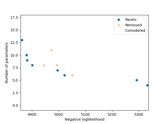
The following plot illustrates all models that have been estimated. Each dot corresponds to a model. The x-coordinate corresponds to the negative log-likelihood. The y-coordinate corresponds to the number of parameters. If the shape of the dot is a circle, it means that it corresponds to a Pareto optimal model. If the shape is a cross, it means that the model has been Pareto optimal at some point during the algorithm and later removed as a new model dominating it has been found.

if can_plot:
    try:
        _ = the_pareto_post.plot(
            label_x='Negative loglikelihood', label_y='Number of parameters'
        )
        plt.show()
    except OptimizationError as e:
        print(f'No plot available: {e}')