Simulation of a mixture model

Simulation of the mixture model, with estimation of the integration error.

author:

Michel Bierlaire, EPFL

date:

Sun Apr 9 17:47:42 2023

import sys
import numpy as np
import biogeme.biogeme as bio
from biogeme import models
import biogeme.results as res
from biogeme.exceptions import BiogemeError
from biogeme.expressions import Beta, bioDraws, MonteCarlo

See the data processing script: Data preparation for Swissmetro.

from swissmetro_data import (
    database,
    CHOICE,
    SM_AV,
    CAR_AV_SP,
    TRAIN_AV_SP,
    TRAIN_TT_SCALED,
    TRAIN_COST_SCALED,
    SM_TT_SCALED,
    SM_COST_SCALED,
    CAR_TT_SCALED,
    CAR_CO_SCALED,
)

try:
    import matplotlib.pyplot as plt

    PLOT = True
except ModuleNotFoundError:
    print('Install matplotlib to see the distribution of integration errors.')
    print('pip install matplotlib')
    PLOT = False

Parameters to be estimated.

ASC_CAR = Beta('ASC_CAR', 0, None, None, 0)
ASC_TRAIN = Beta('ASC_TRAIN', 0, None, None, 0)
ASC_SM = Beta('ASC_SM', 0, None, None, 1)
B_COST = Beta('B_COST', 0, None, None, 0)

Define a random parameter, normally distributed, designed to be used for Monte-Carlo simulation.

B_TIME = Beta('B_TIME', 0, None, None, 0)

It is advised not to use 0 as starting value for the following parameter.

B_TIME_S = Beta('B_TIME_S', 1, None, None, 0)
B_TIME_RND = B_TIME + B_TIME_S * bioDraws('B_TIME_RND', 'NORMAL')

Definition of the utility functions.

V1 = ASC_TRAIN + B_TIME_RND * TRAIN_TT_SCALED + B_COST * TRAIN_COST_SCALED
V2 = ASC_SM + B_TIME_RND * SM_TT_SCALED + B_COST * SM_COST_SCALED
V3 = ASC_CAR + B_TIME_RND * CAR_TT_SCALED + B_COST * CAR_CO_SCALED

Associate utility functions with the numbering of alternatives.

V = {1: V1, 2: V2, 3: V3}

Associate the availability conditions with the alternatives.

av = {1: TRAIN_AV_SP, 2: SM_AV, 3: CAR_AV_SP}

The estimation results are read from the pickle file.

try:
    results = res.bioResults(pickleFile='saved_results/b05_estimation_results.pickle')
except BiogemeError:
    print(
        'Run first the script 05normalMixture.py in order to generate the '
        'file 05normalMixture.pickle.'
    )
    sys.exit()

Conditional to B_TIME_RND, we have a logit model (called the kernel)

prob = models.logit(V, av, CHOICE)

We calculate the integration error. Note that this formula assumes independent draws, and is not valid for Halton or antithetic draws.

integral = MonteCarlo(prob)
integralSquare = MonteCarlo(prob * prob)
variance = integralSquare - integral * integral
error = (variance / 2.0) ** 0.5

And the value of the individual parameters.

numerator = MonteCarlo(B_TIME_RND * prob)
denominator = integral

simulate = {
    'Numerator': numerator,
    'Denominator': denominator,
    'Integral': integral,
    'Integration error': error,
}

Create the Biogeme object.

biosim = bio.BIOGEME(database, simulate)
biosim.modelName = 'b05normal_mixture_simul'

Simulate the requested quantities. The output is a Pandas data frame.

simresults = biosim.simulate(results.getBetaValues())

95% confidence interval on the log likelihood.

simresults['left'] = np.log(
    simresults['Integral'] - 1.96 * simresults['Integration error']
)
simresults['right'] = np.log(
    simresults['Integral'] + 1.96 * simresults['Integration error']
)

/Users/bierlair/venv312/lib/python3.12/site-packages/pandas/core/arraylike.py:396: RuntimeWarning: invalid value encountered in log
  result = getattr(ufunc, method)(*inputs, **kwargs)

print(f'Log likelihood: {np.log(simresults["Integral"]).sum()}')

Log likelihood: -5216.316731053104

print(
    f'Integration error for {biosim.number_of_draws} draws: '
    f'{simresults["Integration error"].sum()}'
)

Integration error for 500 draws: 700.5475488837479

print(f'In average {simresults["Integration error"].mean()} per observation.')

In average 0.10350879859393439 per observation.

95% confidence interval

print(
    f'95% confidence interval: [{simresults["left"].sum()} - '
    f'{simresults["right"].sum()}]'
)

95% confidence interval: [-7529.657511926459 - -2766.3838983681285]

Post processing to obtain the individual parameters.

simresults['beta'] = simresults['Numerator'] / simresults['Denominator']

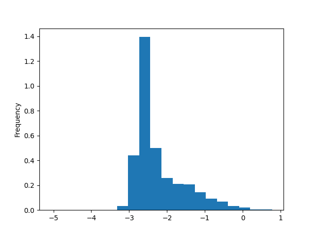
Plot the histogram of individual parameters

if PLOT:
    simresults['beta'].plot(kind='hist', density=True, bins=20)

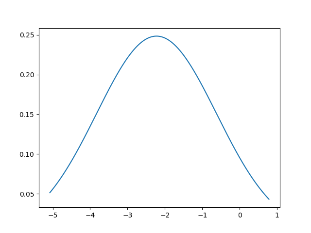
Plot the general distribution of beta

def normalpdf(val, mu=0.0, std=1.0):
    """
    Calculate the pdf of the normal distribution, for plotting purposes.

    """
    d = -(val - mu) * (val - mu)
    n = 2.0 * std * std
    a = d / n
    num = np.exp(a)
    den = std * 2.506628275
    p = num / den
    return p

betas = results.getBetaValues(['B_TIME', 'B_TIME_S'])
x = np.arange(simresults['beta'].min(), simresults['beta'].max(), 0.01)

if PLOT:
    plt.plot(x, normalpdf(x, betas['B_TIME'], betas['B_TIME_S']), '-')
    plt.show()