Calculation of willingness to pay

We calculate and plot willingness to pay. Details about this example are available in Section 4 of Bierlaire (2018) Calculating indicators with PandasBiogeme

author:

Michel Bierlaire, EPFL

date:

Wed Apr 12 20:57:00 2023

import sys

try:
    import matplotlib.pyplot as plt

    can_plot = True
except ModuleNotFoundError:
    can_plot = False
import biogeme.biogeme as bio
import biogeme.exceptions as excep
import biogeme.results as res

from biogeme.expressions import Derive
from optima_data import database, normalized_weight
from scenarios import scenario

Obtain the specification for the default scenario The definition of the scenarios is available in Specification of a nested logit model.

V, _, _, _ = scenario()

V_PT = V[0]
V_CAR = V[1]

Calculation of the willingness to pay using derivatives.

WTP_PT_TIME = Derive(V_PT, 'TimePT') / Derive(V_PT, 'MarginalCostPT')
WTP_CAR_TIME = Derive(V_CAR, 'TimeCar') / Derive(V_CAR, 'CostCarCHF')

Formulas to simulate.

simulate = {
    'weight': normalized_weight,
    'WTP PT time': WTP_PT_TIME,
    'WTP CAR time': WTP_CAR_TIME,
}

Create the Biogeme object.

the_biogeme = bio.BIOGEME(database, simulate)

Read the estimation results from the file.

try:
    results = res.bioResults(pickleFile='saved_results/b02estimation.pickle')
except excep.BiogemeError:
    sys.exit(
        'Run first the script b02estimation.py in order to generate '
        'the file b02estimation.pickle.'
    )

simulated_values is a Pandas dataframe with the same number of rows as the database, and as many columns as formulas to simulate.

simulated_values = the_biogeme.simulate(results.getBetaValues())
simulated_values

	weight	WTP PT time	WTP CAR time
0	0.886023	0.040308	0.040308
2	0.861136	0.040308	0.040308
3	0.861136	0.040308	0.040308
4	0.957386	0.111499	0.111499
5	0.861136	0.040308	0.040308
...	...	...	...
2259	2.036009	0.040308	0.040308
2261	0.861136	0.111499	0.111499
2262	0.861136	0.111499	0.111499
2263	0.957386	0.040308	0.040308
2264	0.957386	0.040308	0.040308

1906 rows × 3 columns

Note the multiplication by 60 to have the valus of time per hour and not per minute.

wtpcar = (60 * simulated_values['WTP CAR time'] * simulated_values['weight']).mean()

Calculate confidence intervals

b = results.getBetasForSensitivityAnalysis(the_biogeme.free_beta_names())

Returns data frame containing, for each simulated value, the left and right bounds of the confidence interval calculated by simulation.

left, right = the_biogeme.confidenceIntervals(b, 0.9)

Lower bounds of the confidence intervals

left

	weight	WTP PT time	WTP CAR time
0	0.886023	0.011110	0.011110
2	0.861136	0.011110	0.011110
3	0.861136	0.011110	0.011110
4	0.957386	0.069673	0.069673
5	0.861136	0.011110	0.011110
...	...	...	...
2259	2.036009	0.011110	0.011110
2261	0.861136	0.069673	0.069673
2262	0.861136	0.069673	0.069673
2263	0.957386	0.011110	0.011110
2264	0.957386	0.011110	0.011110

1906 rows × 3 columns

Upper bounds of the confidence intervals

right

	weight	WTP PT time	WTP CAR time
0	0.886023	0.08798	0.08798
2	0.861136	0.08798	0.08798
3	0.861136	0.08798	0.08798
4	0.957386	0.17001	0.17001
5	0.861136	0.08798	0.08798
...	...	...	...
2259	2.036009	0.08798	0.08798
2261	0.861136	0.17001	0.17001
2262	0.861136	0.17001	0.17001
2263	0.957386	0.08798	0.08798
2264	0.957386	0.08798	0.08798

1906 rows × 3 columns

Lower and upper bounds of the willingness to pay.

wtpcar_left = (60 * left['WTP CAR time'] * left['weight']).mean()
wtpcar_right = (60 * right['WTP CAR time'] * right['weight']).mean()
print(
    f'Average WTP for car: {wtpcar:.3g} ' f'CI:[{wtpcar_left:.3g}, {wtpcar_right:.3g}]'
)

Average WTP for car: 3.96 CI:[1.93, 7.05]

In this specific case, there are only two distinct values in the population: for workers and non workers

print(
    'Unique values:      ',
    [f'{i:.3g}' for i in 60 * simulated_values['WTP CAR time'].unique()],
)

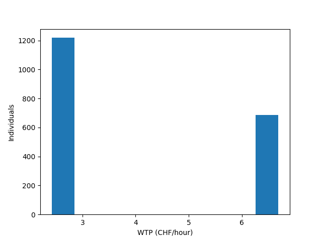
Unique values:       ['2.42', '6.69']

Function calculating the willingness to pay for a group.

def wtp_for_subgroup(the_filter: 'pd.Series[np.bool_]') -> tuple[float, float, float]:
    """
    Check the value for groups of the population. Define a function that
    works for any filter to avoid repeating code.

    :param the_filter: pandas filter

    :return: willingness-to-pay for car and confidence interval
    """
    size = the_filter.sum()
    sim = simulated_values[the_filter]
    total_weight = sim['weight'].sum()
    weight = sim['weight'] * size / total_weight
    _wtpcar = (60 * sim['WTP CAR time'] * weight).mean()
    _wtpcar_left = (60 * left[the_filter]['WTP CAR time'] * weight).mean()
    _wtpcar_right = (60 * right[the_filter]['WTP CAR time'] * weight).mean()
    return _wtpcar, _wtpcar_left, _wtpcar_right

Full time workers.

aFilter = database.data['OccupStat'] == 1
w, l, r = wtp_for_subgroup(aFilter)
print(f'WTP car for workers: {w:.3g} CI:[{l:.3g}, {r:.3g}]')

WTP car for workers: 6.69 CI:[4.18, 10.2]

Females.

aFilter = database.data['Gender'] == 2
w, l, r = wtp_for_subgroup(aFilter)
print(f'WTP car for females: {w:.3g} CI:[{l:.3g}, {r:.3g}]')

WTP car for females: 3.17 CI:[1.29, 6.15]

Males.

aFilter = database.data['Gender'] == 1
w, l, r = wtp_for_subgroup(aFilter)
print(f'WTP car for males  : {w:.3g} CI:[{l:.3g}, {r:.3g}]')

WTP car for males  : 4.96 CI:[2.75, 8.2]

We plot the distribution of WTP in the population. In this case, there are only two values

if can_plot:
    plt.hist(
        60 * simulated_values['WTP CAR time'],
        weights=simulated_values['weight'],
    )
    plt.xlabel('WTP (CHF/hour)')
    plt.ylabel('Individuals')
    plt.show()